In my earlier post, I looked into the VLOOKUP function and its uses. You may also find more examples this post by Colin Legg. Also, Charles Williams had a nice entry on how VLOOKUP performs, and the difference between exact search and approximate search in terms of algorithm.
In this post, I will focus on the INDEX and MATCH functions and how, used together, they can do the same things as the VLOOKUP functions and sometimes more.
Basics
Introduction
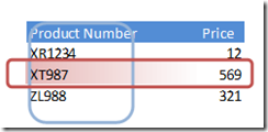
In the following we will use the following reference table, from which we want to extract price information, given some product number.

Suppose we want to get the price corresponding to product number XT987. We will first look for the value XT987 in the Product Number column and will get its relative position within the Product Number range. This is where the MATCH function comes into play.
In our case the formula will look like this:
=MATCH(“XT987”, product_number, 0)
We ask Excel to look for the value XT987 in the Product Number column, performing an exact search (that is what the 0 value stands for.) Excel will return the value 2
.
Once done we will retrieve the price from the same row in the Price column. This is where INDEX comes into play.
In our case the formula will look like this:
=INDEX(price,2)
We ask Excel to return the value found at the 2nd place in the Price column.

This is of course possible to do this in one single formula:
=INDEX(price, MATCH(“XT987”, product_number, 0))
Why use INDEX+MATCH instead of VLOOKUP?
Nesting a MATCH function in an INDEX function does not look as nice or readable as a VLOOKUP formula. So what is it good for?
1. Since we can provide a lookup column (product_number) and a result column (price) independently, we are not limited to using data with the lookup column on the left-hand side of the result column.
This is similar to what the LOOKUP function (not VLOOKUP, not HLOOKUP) can do, except LOOKUP requires your data to be sorted.
2. Actually, we are not even limited to using columns, or ranges. The formula would not change if the lookup and result column were both rows, or one in row one in column. We can also use a formula with hard-coded arrays, if we want:
=INDEX({12,569,321},EQUIV(“XT987”,{“XR134″,”XT987″,”ZL988”},0))
3. The match function supports one additional option for approximate searches, which allows, once again, for more flexibility.
4. Finally, and this is probably the most powerful feature, INDEX returns a reference and not a value. That means, if you used a range for your result column, then you will retrieve a cell reference, which means you can use the result of this formula with functions that take ranges as input values, or with range operators.
The MATCH function
The Syntax
The syntax of the match function is very simple, and will probably remind you of the VLOOKUP syntax.
=MATCH(key_value, lookup_range, lookup_type)
The lookup_value is the value you are looking for. In our example, this will be “XT987”.
The lookup_range will be the range where you are looking for the value. In our case, this will be the column Product Number.
The lookup_type parameter can take the values –1, 0, or 1. When this parameter has the value 0, Excel will perform an exact search. When this parameter is either –1 or 1, Excel will perform an approximate search (more on that later.)
The return value is the position within the lookup range (or array, since MATCH also accepts arrays), where the key value was found.
Lookup types
The look up type parameter accepts 3 values: –1, 0, or 1.
0 means the search will be exact. This corresponds to the search behavior of the VLOOKUP function, when we choose the value FALSE for its last parameter.
1 means the search will be an approximate search, and requires the data to be sorted in ascending order. This corresponds to the default search behavior of the VLOOKUP function, or when we choose the value TRUE for its last parameter.
-1 means the search will be an approximate search, and requires the data to be sorted in descending order. This has no equivalent in the VLOOKUP function.
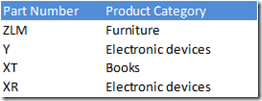
Suppose your data looks like this and you want to search through the Part Number column.

The MATCH function will return the following values, depending on the value provided for the type parameter.

For the type –1, Excel expects data sorted in descending order and, to keep it simple, will return errors most of the time. For the type 0, the value will return an error if the searched value could not be found. For the type 1, Excel will return the last position of the value in the column, or if not found the position of the last available value that is “smaller” than the searched value.
So a value of 0 for the parameter type will return #N/A for a non existing value.
Now, if the data were sorted in descending order

the option –1 would return the following results.

It will return the first value in the list, that is “larger” than the searched value.
The INDEX function
The Syntax
The INDEX function is actually really complex, and would deserve its own post. Basically, it will take up to 4 parameters, and has two syntax forms
=INDEX(matrix, r)
=INDEX(matrix, r, c)
=INDEX(matrix, r, c, range_index)
This function allows you to fetch a reference to the cell on the r-th row of the c-th column of the input matrix. To keep things simple, I will not talk about the last parameter in this post.
One important thing to note, is that the function also allows you to fetch a whole row, a whole column, or even a whole matrix.
For example, the following formula
=INDEX(matrix, 0, 1)
will retrieve the first column of the input matrix.
Optional parameters
Officially, the index function must have at least 2 arguments. However, we may skip any argument past the matrix and the function will still return valid results. For example,
=INDEX(matrix,,1)
(note the two commas) will return the same result as
=INDEX(matrix,0,1)
The following function
=INDEX(column,)
does the same as
=INDEX(column,0)
and will return our input column.
Multiple lookup with INDEX & MATCH
Suppose we have the following table that tracks the price of different products depending on the year.

Now we want to re-use this information in another table. That is, we want to fetch the relevant price, based on some reference to a year value (key_year), and a reference to a product number (key_product).
We will first use the MATCH function to find the first and the last row number for the relevant year, in the Year column.
Let us define a named calculation for the index of the first row where key_year can be found
first_cell_index =MATCH(key_year,year,0)
Let us define a named calculation for the index of the last row where key_year can be found
last_cell_index =MATCH(key_year,year,1)
Given these formulas, and using the fact that INDEX returns cell references, we are now able to fetch the relevant Product Number and Price ranges.
Let us start by using our named calculations in the index functions, to define two new named calculations.
For the first relevant cell in the Product Number range
first_cell_product = INDEX(product_number, first_cell_index )
and for the last cell:
last_cell_product = INDEX(product_number, last_cell_index)
The relevant range can then be constructed by using the range operator “:”. This gives the following formula:
range_product =first_cell_product : last_cell_product
Similarly, we can define the relevant range for the price
first_cell_price = INDEX(price, first_cell_index )
last_cell_price = INDEX(price, last_cell_index )
range_price = first_cell_price : last_cell_price
Using the above named calculations and applying an INDEX + MATCH formula again, we can now match the relevant information for the given key_product.
=INDEX(range_price,
MATCH(key_product, range_product,0)
)


